What is Mixed Factors Analysis ?
In below, we describe a belief introduction of the mixed factors analysis.
For more details, see our papers,
- R.Yoshida, T.Higuchi and S.Imoto (2004), A Mixed Factors Model for Dimension Reduction and Extraction of A Group Structure in Gene Expression Data, Proc. IEEE 3rd Computational Systems Bioinformatics (CSB2004: Refereed Coference), 161-172. * Full text of this paper is available from CSB2004's website.
- R.Yoshida, S.Imoto and T.Higuchi (2005), A Penalized Likelihood Estimation on Transcriptional Module-based Clustering, Proc.1st International Workshop on Data Mining and Bioinformatics (DMBIO 2005: Refereed Conference), Lecture Note in Computer Science vol. 3482, Springer-Verlag, 389-401.
1.Introduction
In gene expression profiling based on microarray experiments, each array
measures expression values of several thousands genes for a tissue sample.
A goal of the cluster analysis is to find groups in a given set of tissue
samples on the basis of a large number of genes. Major difficulty in this
problem is that the number of tissues to be grouped is much smaller than
the dimension of feature vector which is equal to the number of genes involved.
In such a case, conventional model-based clustering using finite mixture
models, e.g. Gaussian mixture, leads to overfitting during the density
estimation process. The mixed factors analysis was originally aimed at
resolving the problem of curse of high-dimensionality faced at gene expression
analysis. A parametric model referred to as the mixed factors model is
a central in this context and performs a parsimonious parameterization
of Gaussian mixture model. As a result of this modeling, we can avoid the
occurrence of overfitting even when the dimension of data is more than
several thousands and the number of sample is less than one hundred.
2.Mixed Factors Model
We let x ( j ) be a d-dimensional feature vector which contains the expression values of d genes for the j-th tissue sample ( j = 1,・・・,N ). In gene expression profiling, the dimension of data typically rangies
from 100 to 10000. A basic idea underlying the mixed factor analysis is
to relate the high-dimensional feature vectors to the q-dimensional factor
variables f ( j ), j = 1,・・・,N in the following way:
- x( j ) = A f( j ) + e( j ). ·······(1).
.
Here q<d, and the e( j ) is the Gaussian observational noise as e( j ) 〜 N(0, r I). The matrix A of order d ×q contains the factor loadings.
A key idea of the mixed factors modeling is to parsimoniously describe
the group structure of data throughout the factor variables. To this end,
we assume that the factor variables are distributed according to the finite
mixture model as
- P( f( j ) ) = b_1 H( f ( j ) ; u_1 , V_1)+ ········· + b_G H( f ( j ) ; u_G , V_G). ······ (2)
Here, the H( f( j ) ; u_g, V_g) denotes the Gaussian density function with mean vector u_g and covariance matrix V_g. The mixing proportions are given by b_1, ・・・,b_G. We construct the mixed factors model by combining (1) and (2).
The mixed factors model represents the unconditional distribution of data
by the G-components Gaussian mixture with the following parsimonious parameterization:
- P( x( j ) ) = b_1 H( x ( j ) ; m_1 , D_1)+ ········· + b_G H( x ( j ) ; m_G , D_G),
- Group Mean; m_g = A u_g,
- Group Covariance Matrix; D_g = A V_g A' + r I.
This parameterization possibly avoids the overfitting occurred in the parameter estimation by choosing an appropriate factor dimension q despite of the quite huge dimension of data.
Remark:Parameter Constrains
Parameters to be estimated from data consist of A, r and b_g, u_g, V_g for all g. However, a direct estimation of these parameters leads to the
lack of identifiability due to the issue of rotational ambiguity. For detail,
see Yoshida et al. (2004). To avoid such problem, we impose q ×q restrictions on the parameters; (a) diagonality of the covariance
matrix, V_g = diag(v_{1g},・・・v_{qg}); (b) orthogonality of factor loadings A' A= I. Imposing orthogonality on the factor loading matrix offers a linear mapping
of data, A'x ( j ), onto the q-dimensional subspace, having an observational equation,
- A'x( j ) = f( j ) + A'e( j ).
This equation states the fact that the compressed data A'x( j ) are distributed according to the Gaussian mixture as
- P( A'x( j ) ) =b_1 H( A'x( j );u_1, V_1+rI ) + ·········· + b_G H( A'x( j );u_G, V_G+rI ). ······ (3).
This expression gives us an interesting view about the mixed factors model. Roughly speaking, in the parameter estimation, q-directions in the projection matrix A should be chosen so that the compressed data are likely to be the Gaussian mixture in the form of (3). More formal discussions including the linkage to the Fisher's discriminant analysis and the principal component analysis are given in our paper Yoshida et al. (2005).
3.Module Transcriptional-based Clusters
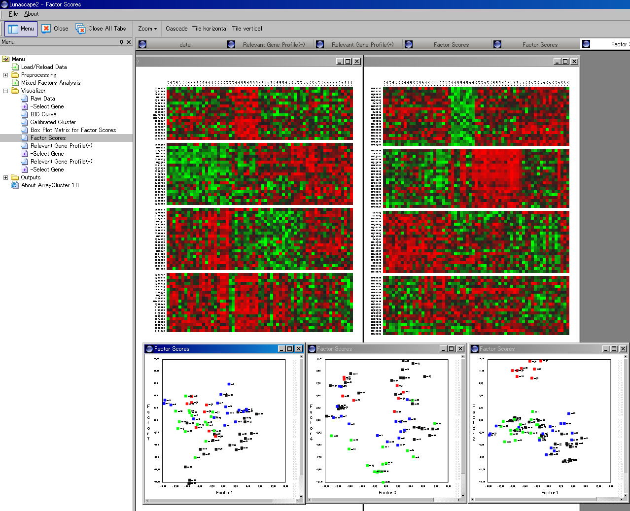
In cellular systems, each gene is expressed either by itself or in combination with some other genes. Figure 1 displays the expression patterns of a variety of small round blue cell tumor tissues against to the 16 module
gene sets. These sets are automatically identified with the mixed factors
analysis. All genes in a particular set tend to exhibit very similar expression
patterns.
In the mixed factors analysis, the expression patterns of the existing
transcriptional modules are extracted and compressed into the low-dimensional
factor space via q-variates in A'x( j ) as follows:
- If (A'x( j ))_ij is positioned far from zero, the j-th gene captures a large effect on the i-th module.
- In contrast, the influence of gene with the(A'x( j ))_ij lying a region close to zero is removed.
4.Mixed Factors Analysis
For a given dataset, the mixed factors model can be fitted based on the maximum likelihood estimation. The ArrayCluster computes the maximum likelihood estimator by using the EM algorithm. The algorithmic details are omitted here, see Yoshida et al.(2004) .
Once the parameter has been estimated, our method offers some useful applications to gene expression analysis. The following is a flowchart of the mixed factors analysis:
- Determination of the number of clusters and the factor dimension (the number of module transcriptionals). In ArrayCluster, these tasks are addressed with the Bayesian information criterion (BIC).
- Data visualization via the estimation of the factor scores. In ArrayCluster, this turns to computing the posterior mean of factor variables i.e. E [ f ( j ) | x( j ) ]. .
- Clustering based on the Bayes rule, i.e. "Group of x( j )" = argmax_h Pr {A'x( j ) in Group h }.
- Identification of module transcriptional genes that are relevant to the calibrated clusters. In ArrayCluster, a number of genes are selected to have top L of the highest positive correlation (negative correlation) with each element of factor vector. Thus, total 2q transcriptionals are identified. The ArrayCluster also offers an option for a number of relevant genes to be listed at a module.
- Missing imputation.
Figure 1: A number of module transcriptionals identified by the mixed factors analysis
This work was carried out in the laboratory of Tomoyuki Higuchi, The Institute of Statistical Mathematics, Research Organization of Information and Systems, and the laboratory of
Satoru Miyano, DNA Information Analysis, Human Genome Center, Institute
of Medical Science, University of Tokyo.
Developers; Tomoyuki Higuchi, Ryo Yoshida, Seiya Imoto, Satoru Miyano
Copyright; (C) 2005- Tomoyuki Higuchi (C) 2005- Ryo Yoshida (C) 2005- Seiya Imoto (C) 2005-
Satoru Miyano (C) 2005- The Institute of Statistical Mathematics, Research Organization of Information and Systems (C) 2005- Human Genome
Center, Institute of Medical Science, University of Tokyo